Day 7 Handy Haversacks

This is my attempt to solve Day 7.

sample <- read_lines("samples/day_07_sample.txt")
actual <- read_lines("inputs/day_07_input.txt")

7.1 Part 1

I think today’s problem is naturally solved with using graph’s, so I’m going to use the {igraph} package. The easiest way to create a graph is to first create a data frame that contains the columns from and to that indicate which edges are in the graph. Any additional columns will be added as properties to the edge.

convert_input_to_tibble <- function(input) {
  input %>%
    # we don't need to keep the word's "bag" or "bags". In our data these words
    # always have a space before, and sometimes have a "." at the end. We can
    # use the following regex to remove these words
    str_remove_all(" bags?\\.?") %>%
    # we can now split our data at the word "contains"
    unglue_data("{from} contain {contains}") %>%
    # now we can split the contains column by comma's
    mutate(across(contains, str_split, ", ")) %>%
    # and expand the nested "contains" column
    unnest_longer(contains) %>%
    # handle edge case: if the string is no other need to insert a 0 at the start
    mutate(across(contains, ~if_else(.x == "no other", "0 no other", .x))) %>%
    # now we can split the contains column into the "n" part and the "to" part
    separate(contains, c("n", "to"), "(?<=\\d) ", convert = TRUE) %>%
    # reorder the columns
    select(from, to, n)
}
sample_df <- convert_input_to_tibble(sample)
actual_df <- convert_input_to_tibble(actual)
sample_df

## # A tibble: 15 x 3
##    from         to               n
##    <chr>        <chr>        <int>
##  1 light red    bright white     1
##  2 light red    muted yellow     2
##  3 dark orange  bright white     3
##  4 dark orange  muted yellow     4
##  5 bright white shiny gold       1
##  6 muted yellow shiny gold       2
##  7 muted yellow faded blue       9
##  8 shiny gold   dark olive       1
##  9 shiny gold   vibrant plum     2
## 10 dark olive   faded blue       3
## 11 dark olive   dotted black     4
## 12 vibrant plum faded blue       5
## 13 vibrant plum dotted black     6
## 14 faded blue   no other         0
## 15 dotted black no other         0

We can create a graph using the graph_from_data_frame() function:

sample_g <- graph_from_data_frame(sample_df)
sample_g

## IGRAPH fd1e49d DN-- 10 15 -- 
## + attr: name (v/c), n (e/n)
## + edges from fd1e49d (vertex names):
##  [1] light red   ->bright white light red   ->muted yellow
##  [3] dark orange ->bright white dark orange ->muted yellow
##  [5] bright white->shiny gold   muted yellow->shiny gold  
##  [7] muted yellow->faded blue   shiny gold  ->dark olive  
##  [9] shiny gold  ->vibrant plum dark olive  ->faded blue  
## [11] dark olive  ->dotted black vibrant plum->faded blue  
## [13] vibrant plum->dotted black faded blue  ->no other    
## [15] dotted black->no other

and visualise this graph using {igraph}:

ggraph(sample_g, layout = "igraph", algorithm = "nicely") +
  geom_edge_link(aes(label = n), 
                 angle_calc = "along",
                 label_dodge = unit(2.5, "mm"),
                 arrow = arrow(length = unit(3, "mm")), 
                 end_cap = circle(10, "mm")) + 
  geom_node_label(aes(label = str_replace(name, " ", "\n")))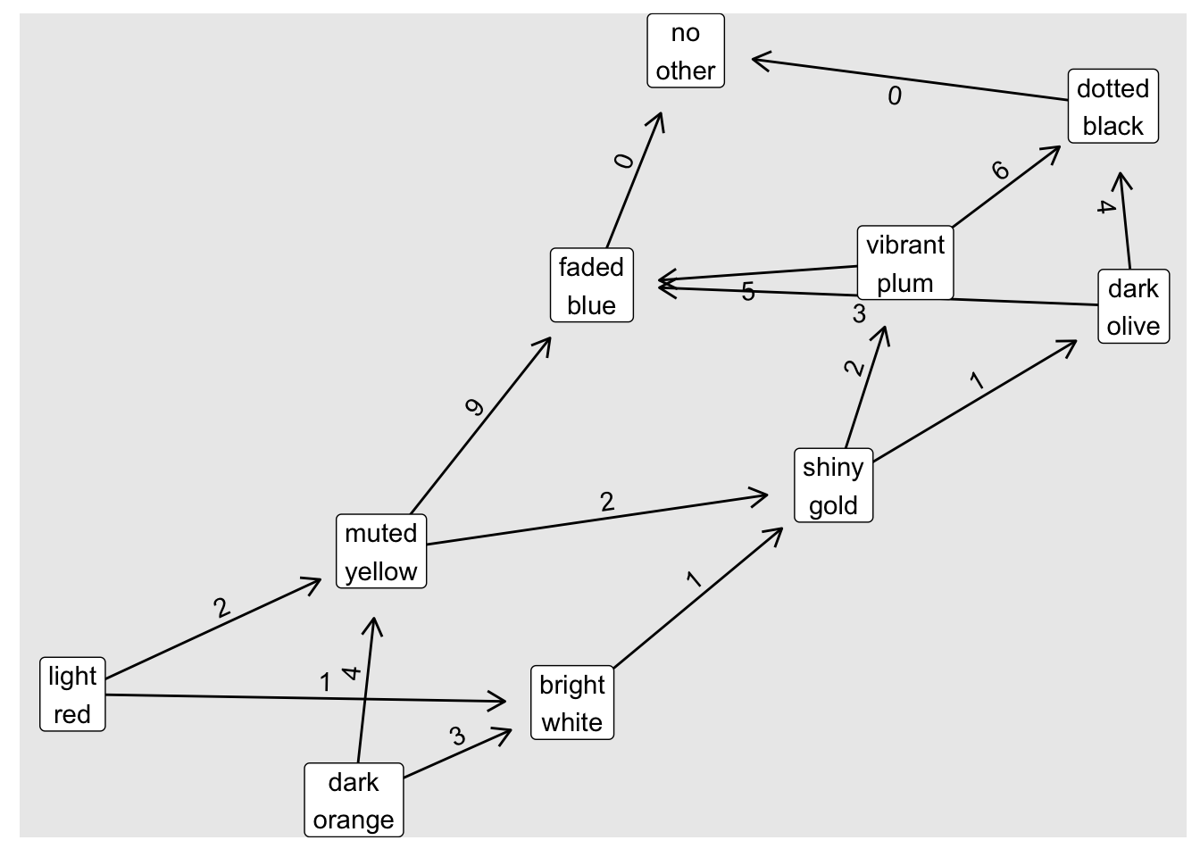

Our challenge is to find all of the vertices that have a path in to “shiny gold”. The subcomponent() function can tell us all of the vertices in a graph which reach a given vertex. We can simply take the length of this subcomponent and subtract 1 (as the subcomponent includes “shiny gold”).

length(subcomponent(sample_g, "shiny gold", "in")) - 1 == 4

## [1] TRUE

We now just need to solve for the actual data.

actual_g <- graph_from_data_frame(actual_df)
length(subcomponent(actual_g, "shiny gold", "in")) - 1

## [1] 278

7.2 Part 2

Part 2 sounds like a recursive function. We can first find the subgraph that includes all of the vertices from “shiny gold”. We can then convert this graph to an adjacency matrix and iterate through each vertex, recursively calling a function that sums how many bags this bag will contain.

part_2 <- function(input) {
  sg <- induced_subgraph(input, subcomponent(input, "shiny gold", "out"))
  am <- as_adjacency_matrix(sg, attr = "n", sparse = FALSE)
  
  fn <- function(am, v = "shiny gold", n = 1) {
    a <- am[v, ] * n
    a <- a[a > 0] # keep as separate step, otherwise can end up with just scalar
    
    # now, iterate over each item in a and recursively call this function
    sum(map_dbl(names(a), ~fn(am, .x, a[[.x]]))) + sum(a)
  }
  
  # call this function on the base case
  fn(am)
}

We can test that our function works against the sample case:

part_2(sample_g) == 32

## [1] TRUE

A second sample is provided, so we can test against that also:

c("shiny gold bags contain 2 dark red bags.",
  "dark red bags contain 2 dark orange bags.",
  "dark orange bags contain 2 dark yellow bags.",
  "dark yellow bags contain 2 dark green bags.",
  "dark green bags contain 2 dark blue bags.",
  "dark blue bags contain 2 dark violet bags.",
  "dark violet bags contain no other bags.") %>%
  convert_input_to_tibble() %>%
  graph_from_data_frame() %>%
  part_2() == 126

## [1] TRUE

Now we can run against the actual data:

part_2(actual_g)

## [1] 45157

7.3 Extra: alternative solution to part 2

We could also solve part 2 by iterating through each vertex and finding the incident edges and adjacent vertices. We multiply the edge weight (ie$n) by the current value of n, sum these values and add n back in to the total. This gives us the total number of bags, including the initial bag, so we need to subtract 1 from this answer.

part_2_alt <- function(g, v, n) {
  ie <- incident_edges(g, v, "out")[[1]]
  vn <- ends(g, ie)[, 2]
  sum(map2_dbl(vn, ie$n * n, part_2_alt, g = g)) + n
}

We can now verify that this alternative function works as above.

part_2_alt(sample_g, "shiny gold", 1) - 1 == part_2(sample_g)

## [1] TRUE

part_2_alt(actual_g, "shiny gold", 1) - 1 == part_2(actual_g)

## [1] TRUE

---

Elapsed Time: 2.362s